Exploration of Mixture g-Priors BMA Variable Selection in Generalized Linear Model with Microarray Data
Bayesian model average is a well-known method that provides a coherent mechanism for accounting for the model uncertainty [1]. In BMA, we place a prior probability $\pi$ on the model in the model space such that:
\[\begin{aligned} &\pi\left(\mathcal{M}_{m}\right)>0 \\ &\sum_{m=1}^{M} \pi\left(\mathcal{M}_{m}\right)=1 \end{aligned}\]The BMA framework can be written as:
\[\begin{array}{lr} \begin{aligned} X_{i} \mid \boldsymbol{\theta}, \mathcal{M}_{m} & \stackrel{\text { ind }}{\sim} f_{m}\left(x_{i} \mid \boldsymbol{\theta}_{m}\right), & i=1, \ldots, n \\ \boldsymbol{\theta}_{m} & \stackrel{\text { ind }}{\sim} g_{m}\left(\boldsymbol{\theta}_{m}\right), & m=1, \ldots, M \\ \mathcal{M}_{m} & \sim \pi\left(\mathcal{M}_{m}\right) & \end{aligned}&(1) \end{array}\]In the gaussian regression model setting, there are already many well documented BMA variable selection methods such as mixtures of g-priors [2] and spike and slab regression model [3]. These methods can also apply to the high dimensional $p » n$ gaussian regression problem. Although many related works are also proposed in the generalized linear model settings, it is not widely implemented as in the gaussian regression setting. Moreover, in the micro array dataset, We prefer to select a relatively smaller size of gene signatures, but many of the current variable selection methods produce uncertainty in gene selection. The results of selected genes may be different every time running the variable selection method. Therefore, we will mainly explore the mixtures of g-priors method that proposed by Li and Clyde [4]. and the effects of different choice of $g$ and model selection priors to the high dimensional microarray two-class problem. In R, Clyde et al. had implemented mixtures of g-priors methods using Bayesian Adaptive Sampling in the package called BAS. The major data analysis part of this project will be conducted by this package [5].
Check the code for this paper: https://github.com/noblegasss/gprior_BMA
Prior Settings
Assume that the column of $\mathbf{X}_{\mathcal{M}}$ have been centered. In the gaussian regression settings, the general framework of Zellner’s g-priors BMA assigns a Jeffrey’s prior [2,6] is
\[\begin{array}{lr} \begin{aligned} (\mathbf{Y} \mid \boldsymbol{\beta}, \mathcal{M}) & \sim \mathbf{N}_{n}\left(\mathbf{X}_{\mathcal{M}} \boldsymbol{\beta}_{\mathcal{M}} + \mathbf{1}_n\alpha, \sigma^{2} \mathbf{I}_{n}\right) \\ \boldsymbol{\beta}_{\mathcal{M}} & \sim \mathrm{N}_{p_{\mathcal{M}}}\left(\mathbf{0}, g \sigma^{2} (\mathbf{X}_{\mathcal{M}}^{\top}\mathbf{X}_{\mathcal{M}})^{-1}\right) \\ (\sigma^2 ,\alpha)& \sim \frac{1}{\sigma^2} \end{aligned} & (2) \end{array}\]In the generalized linear model setting, $\mathbf{Y}$ has a density in the exponential family [7]
\[\begin{array}{lr} p\left(Y_{i}\right)=\exp \left\{\frac{Y_{i} \theta_{i}-b\left(\theta_{i}\right)}{a\left(\phi_{0}\right)}+c\left(Y_{i}, \phi_{0}\right)\right\}, \quad i=1, \ldots, n, & (3) \end{array}\]where \(\theta_{i}=\theta\left(\eta_{\mathcal{M}, i}\right), \text { and } \eta_{\mathcal{M}}=\mathbf{1}_{n} \alpha+\mathbf{X}_{\mathcal{M}} \beta_{\mathcal{M}}\)
Chen and Ibrahim described an improper flat prior for $\beta_{\mathcal{M}}$ [8]
\[\begin{array}{lr} f\left(\boldsymbol{\beta}_{\mathcal{M}} \mid \boldsymbol{y}_{0}, g, \mathcal{M}\right) \propto \exp \left\{\frac{1}{g \phi} \sum_{i=1}^{n}\left[h(0) w_{i} \theta_{i}-w_{i} b\left(\theta_{i}\right)\right]\right\} & (4) \end{array}\]This improper distribution had been justified to converges to the normal distribution when $n \rightarrow \infty$ [9]
\[\begin{array}{lr} \boldsymbol{\beta}_{\mathcal{M}} \mid g, \mathcal{M} \sim \mathrm{N}_{p_{\mathcal{M}}}\left(\mathbf{0}_{p_{\mathcal{M}}}, g c\left(\boldsymbol{X}_{\mathcal{M}}^{\top} \boldsymbol{X}_{\mathcal{M}}\right)^{-1}\right), & (5) \end{array}\]where $c$ is inverse of the unit information $\mathcal{I}(\eta)=-\mathbb{E}\left[\partial^{2} \log p\left(Y \mid \eta, \mathcal{M}_{\varnothing}\right) / \partial \eta^{2}\right]$ under the null model.
Moreover, Li and Clyde proposed a local information metric g-prior [4]
\[\begin{array}{lr} \boldsymbol{\beta}_{\mathcal{M}} \mid g, \mathcal{M}\sim \mathrm{N}\left(\mathbf{0}, g \cdot \mathcal{J}_{n}\left(\hat{\boldsymbol{\beta}}_{\mathcal{M}}\right)^{-1}\right), & (6) \end{array}\]where
\[\begin{aligned} \mathcal{J}_{n}\left(\hat{\boldsymbol{\beta}}_{\mathcal{M}}\right)&=\mathbf{X}_{\mathcal{M}}^{T}\left(\mathbf{I}_{n}-\mathcal{P}_{\mathbf{1}_{n}}\right)^{T} \mathcal{J}_{n}\left(\hat{\boldsymbol{\eta}}_{\mathcal{M}}\right)\left(\mathbf{I}_{n}-\mathcal{P}_{\mathbf{1}_{n}}\right) \mathbf{X}_{\mathcal{M}} \\ \mathcal{J}_{n}\left(\hat{\alpha}_{\mathcal{M}}\right)&=\mathbf{1}_{n}^{T} \mathcal{J}_{n}\left(\hat{\boldsymbol{\eta}}_{\mathcal{M}}\right) \mathbf{1}_{n}\\ \mathcal{J}_{n}\left(\hat{\eta}_{\mathcal{M}}\right)&=\operatorname{diag}\left(d_{i}\right) \text { where } d_{i}=-Y_{i} \theta^{\prime \prime}\left(\hat{\eta}_{\mathcal{M}, i}\right)+(b \circ \theta)^{\prime \prime}\left(\hat{\eta}_{\mathcal{M}, i}\right) \text { for } i=1, \ldots, n,\\ \text{and } \mathcal{P}_{\mathbf{1}_{n}}&=\mathbf{1}_{n}\left(\mathbf{1}_{n}^{T} \mathcal{J}_{n}\left(\hat{\boldsymbol{\eta}}_{\mathcal{M}}\right) \mathbf{1}_{n}\right)^{-1} \mathbf{1}_{n}^{T} \mathcal{J}_{n}\left(\hat{\boldsymbol{\eta}}_{\mathcal{M}}\right) \end{aligned}\]In particular, the paper discussed the cases that data separation in binary regression and nonfull-rank design matrics for GLM with known dispersion. For $\mathbf{X}_{\mathcal{M}}$ is not full rank, that is,
\(\text{rank}(\mathbf{X}_{\mathcal{M}}) = \rho_{\mathcal{M}} < p_{\mathcal{M}}\),
suppose we have another \(\mathbf{X}_{\mathcal{M}'} \text{ contains } \rho_\mathcal{M}\), such that \(\mathcal{C}(\mathbf{X}_{\mathcal{M}'}) = \mathcal{C}(\mathbf{X}_{\mathcal{M}})\). Then \(\mathcal{J}_{n}\left(\hat{\eta}_{\mathcal{M}}\right)\) is unique and positive definite for the fact that
\(\hat{\eta}_{\mathcal{M}}=\mathbf{1}_{n} \hat{\alpha}_{\mathcal{M}}+\mathbf{X}_{\mathcal{M}} \hat{\boldsymbol{\beta}}_{\mathcal{M}}=\mathbf{1}_{n} \hat{\alpha}_{\mathcal{M}^{\prime}}+\mathbf{X}_{\mathcal{M}^{\prime}} \hat{\boldsymbol{\beta}}_{\mathcal{M}^{\prime}}\) [4].
Therefore, the g-prior (6) does not suffered from singularity problem.
Posterior and Bayesian Factor
The section 2.2 and 2.3 are all derived and mentioned in the Li and Clyde’s paper [4]. Here we just present the major results of the paper. Based on the g-prior (6), the Laplace approximation yields to the approximate posterior distribution
\[\begin{array}{lr} \begin{array}{l} \boldsymbol{\beta}_{\mathcal{M}} \mid \mathbf{Y}, \mathcal{M}, g \stackrel{D}{\longrightarrow} \mathrm{N}\left(\frac{g}{1+g} \hat{\boldsymbol{\beta}}_{\mathcal{M}}, \frac{g}{1+g} \mathcal{J}_{n}\left(\hat{\boldsymbol{\beta}}_{\mathcal{M}}\right)^{-1}\right) \\ \alpha \mid \mathbf{Y}, \mathcal{M} \stackrel{D}{\longrightarrow} \mathrm{N}\left(\hat{\alpha}_{\mathcal{M}}, \mathcal{J}_{n}\left(\hat{\alpha}_{\mathcal{M}}\right)^{-1}\right) \end{array} & (7) \end{array}\]The marginal likelihood derived under an integrated Laplace approximation is
\[\begin{array}{lr} \begin{aligned} p(\mathbf{Y} \mid \mathcal{M}, g)=& \int p\left(\mathbf{Y} \mid \boldsymbol{\beta}_{\mathcal{M}}, \mathcal{M}\right) p\left(\boldsymbol{\beta}_{\mathcal{M}} \mid \mathcal{M}, g\right) d \boldsymbol{\beta}_{\mathcal{M}} \\ & \propto p\left(\mathbf{Y} \mid \hat{\alpha}_{\mathcal{M}}, \hat{\boldsymbol{\beta}}_{\mathcal{M}}, \mathcal{M}\right) \mathcal{J}_{n}\left(\hat{\alpha}_{\mathcal{M}}\right)^{-\frac{1}{2}}(1+g)^{-\frac{p_{M}}{2}} \times \exp \left\{-\frac{Q_{\mathcal{M}}}{2(1+g)}\right\}, \end{aligned} & (8) \end{array}\]where \(Q_{\mathcal{M}}=\hat{\boldsymbol{\beta}}_{\mathcal{M}}^{T} \mathcal{J}_{n}\left(\hat{\boldsymbol{\beta}}_{\mathcal{M}}\right) \hat{\boldsymbol{\beta}}_{\mathcal{M}}\).
Therefore, we can derived the closed-form Bayes factor by the g-prior (6)
\[\begin{array}{lr} \mathrm{BF}_{\mathcal{M}: \mathcal{M}_{\varnothing}}=\frac{p(\mathbf{Y} \mid \mathcal{M}, g)}{p\left(\mathbf{Y} \mid \mathcal{M}_{\varnothing}\right)}=\exp \left\{\frac{z_{\mathcal{M}}}{2}\right\}\left[\frac{\mathcal{J}_{n}\left(\hat{\alpha}_{\mathcal{M}_{\varnothing}}\right)}{\mathcal{J}_{n}\left(\hat{\alpha}_{\mathcal{M}}\right)}\right]^{\frac{1}{2}} \times(1+g)^{-\frac{p_{M}}{2}} \exp \left\{-\frac{Q_{\mathcal{M}}}{2(1+g)}\right\} & (9) \end{array}\]where \(z_{\mathcal{M}}=2 \log \left\{\frac{p\left(\mathbf{Y} \mid \hat{\alpha}_{\mathcal{M}}, \hat{\boldsymbol{\beta}}_{\mathcal{M}}, \mathcal{M}\right)}{p\left(\mathbf{Y} \mid \hat{\alpha}_{\mathcal{M}_{\varnothing}}, \mathcal{M}_{\varnothing}\right)}\right\}\)
g-Priors Selection
Liang et al. discussed in the paper that fixed values of g would lead to some undesirable features – Bartleet’s Paradox and Information Paradox [2]. Therefore, the mixtures of g-priors that lead to closed form expressions were proposed. Li and Clyde further adopted a compound confluent hypergeometric distributions (CCH) to unify the existing mixtures of g-priors [4]. Let $u$ be the shrinkage factor $1/(1+g)$, then $u$ follows a truncated CCH prior distribution
\[\begin{array}{lr} p(u \mid t, q, r, s, v, \kappa)= \frac{v^{t} \exp (s / v)}{B(t, q) \Phi_{1}(q, r, t+q, s / v, 1-\kappa)} \times \frac{u^{t-1}(1-v u)^{q-1} e^{-s u}}{[\kappa+(1-\kappa) v u]^{r}} \mathbf{1}_{\left\{0<u<\frac{1}{v}\right\}}, & (10) \end{array}\]where $t>0, q>0, r \in \mathbb{R}, s \in \mathbb{R}, v \geq 1$, and $\kappa>0$. The prosterior distribution of $u$ under $\mathcal{M}$ is also a tCCH distribution
\[\begin{array}{lr} u \mid \mathbf{Y}, \mathcal{M} \stackrel{D}{\longrightarrow} \operatorname{tCCH}\left(\frac{a+p_{\mathcal{M}}}{2}, \frac{b}{2}, r, \frac{s+Q_{\mathcal{M}}}{2}, v, \kappa\right) & (11) \end{array}\]Moreover,the paper proposed a "confluent hypergeometric information criterion" (CHIC) prior based on a modified Bayes factor. Selection of different parameter of CHIC yields different mixture g-priors. Here we list the density of some special cases of the CHIC g-priors that showed better performance in the paper, We will use these g-priors in the data study later.
1. Confluent Hypergeometric (CH) prior [10]
\[\begin{aligned} u& \sim CH\left(\frac{a}{2},\frac{b}{2}, \frac{s}{2} \right)\\ p(u \mid t, q, s)&=\frac{u^{t-1}(1-u)^{q-1} \exp (-s u)}{B(t, q)_{1} F_{1}(t, t+q,-s)} \mathbf{1}_{\{0<u<1\}} \end{aligned}\]where $t>0, q>0, s \in \mathbb{R},$ and
\[{ }_{1} F_{1}(a, b, s)=\frac{\Gamma(b)}{\Gamma(b-a) \Gamma(a)}\int_{0}^{1} z^{a-1}(1-z)^{b-a-1} \exp (s z) d z\]is the Confluent Hypergeometric function [11]. Liang and Clyde suggested to sset a fixed small on $a$ and order of $O(n)$ on $b$.
2. Robust prior [12]
\[p_{r}(u)= a_{r}\left[\rho_{r}\left(b_{r}+n\right)\right]^{a_{r}} \times \frac{u^{a_{r}-1}}{\left[1+\left(b_{r}-1\right) u\right]^{a_{r}+1}} \mathbf{1}_{\left\{0<u<\frac{1}{\rho r\left(b_{r}+n\right)+\left(1-b_{r}\right)}\right\}},\]where $a_{r}>0, b_{r}>0$, and $\rho_{r} \geq b_{r} /\left(b_{r}+n\right)$ The recommended parameters are $a_{r}=0.5, b_{r}=1$ and $\rho_{r}=1 /\left(1+p_{\mathcal{M}}\right)$ [12].
3. Hyper-g prior [2]
\(u \sim \operatorname{Beta}\left(\frac{a_{h}}{2}-1,1\right), \text { where } 2<a_{h} \leq 4,\) where the default setting of $a_h$ is 3.
4. Hyper-g/n prior [2]
\[p(g)=\frac{a_{h}-2}{2 n}\left(\frac{1}{1+g / n}\right)^{a_{h} / 2}, \text { where } 2<a_{h} \leq 4\]5. Truncated Gamma prior [13]
\[u \sim \mathrm{TG}_{(0,1)}\left(a_{t}, s_{t}\right) \Longleftrightarrow p(u)=\frac{s_{t}^{a_{t}}}{\gamma\left(a_{t}, s_{t}\right)} u^{a_{t}-1} e^{-s_{t} u} \mathbf{1}_{\{0<u<1\}}\]This is the gamma fistribution in the $[0,1]$ support.
7. Intrinsic prior [13]
\[g=\frac{n}{p_{\mathcal{M}}+1} \cdot \frac{1}{w}, \quad w \sim \operatorname{Beta}\left(\frac{1}{2}, \frac{1}{2}\right) .\]We also select some other priors that are not contained in the CHIC g-priors.
8. AIC and BIC
\[\begin{aligned} AIC\left(\mathcal{M}\right)&=-2 \log \left(\operatorname{maximized} \operatorname{likelihood} \mid \mathcal{M}\right)+2p_{\mathcal{M}} \\ B I C\left(\mathcal{M}\right)&=-2 \log \left(\operatorname{maximized} \operatorname{likelihood} \mid \mathcal{M}\right)+p_{\mathcal{M}} \log (n) \end{aligned}\]9. Text Bayes Factor [14]
\[\operatorname{TBF}_{\mathcal{M}: \mathcal{M}_{\varnothing}} =\frac{G\left(z_{\mathcal{M}} ; \frac{p_{\mathcal{M}}}{2}, \frac{1}{2(1+g)}\right)}{G\left(z_{\mathcal{M}} ; \frac{p_{\mathcal{M}}}{2}, \frac{1}{2}\right)} =(1+g)^{-\frac{p_{M}}{2}} \exp \left\{\frac{g z_{\mathcal{M}}}{2(1+g)}\right\}\]Data Experimental Results
We used a two-class prostate cancer dataset to conduct our data experiment. The dataset contains 115 observations and 59 of them are considered as prostate cancer and others are normal. The dimension of the dataset is 5357. However, since the time consuming problem with the large p in the model, we only selected the top 10% variation genes in the dataset. The dimension of the dataset is 537 after filtering , which is still considered as a $p > n$ problem.
We first conduct the analysis of different g-priors using two model priors: uniform and beta binomial(1,1). Then we will compare the mixtures of g-priors with two regularization methods (lasso and elastic net).
Model Performance
For each method, we conducted a 10-fold cross validation and recorded the total unique gene selected sum up by the 10 runs of the model. For the selection criterion we used a fixed criterion $P(\beta \neq 0 \mid Y) > 0.01$ for each model. The reason for this criterion we will discuss later. We also calculated the cv brier score and cv error for each method. The results are showed in the Table 1. As in the paper recommended for CH priors, we selected the parameter $a$ = 1/2 or 1, $b$ = $n$ or $p$, $s$ = 0 by default. The b here is acutually recommended to select on the order of $O(n)$. However, here we mainly to see the effects on the large values of $b$. Other g-priors we used are the default setting except for the tested Bayes factor we chose $g = p$ since it does not have a default values of $g$.
| CH0.5n | CH0.5p | CH1n | CH1p | robust | hyper.g | hyper.g.n | TG | TBF | intrinsic | BIC | AIC | |
|---|---|---|---|---|---|---|---|---|---|---|---|---|
| Total number of beta | 33.00 | 21.00 | 20.00 | 19.0 | 43.00 | 44.00 | 39.00 | 96.00 | 23.00 | 36.00 | 1.00 | 54.00 |
| cv.brier | 0.22 | 0.23 | 0.24 | 0.24 | 0.22 | 0.23 | 0.20 | 0.24 | 0.23 | 0.21 | 0.26 | 0.22 |
| cv.error | 0.33 | 0.37 | 0.38 | 0.43 | 0.34 | 0.31 | 0.27 | 0.33 | 0.36 | 0.31 | 0.65 | 0.34 |
| CH0.5n | CH0.5p | CH1n | CH1p | robust | hyper.g | hyper.g.n | TG | TBF | intrinsic | BIC | AIC | |
|---|---|---|---|---|---|---|---|---|---|---|---|---|
| Total number of beta | 357.00 | 296.00 | 346.00 | 289.00 | 453.00 | 461.00 | 100.00 | 449.00 | 255.00 | 415.00 | 1.00 | 301.00 |
| cv.brier | 0.38 | 0.44 | 0.44 | 0.47 | 0.46 | 0.44 | NA | 0.33 | 0.38 | 0.36 | 0.25 | 0.38 |
| cv.error | 0.38 | 0.44 | 0.44 | 0.47 | 0.48 | 0.52 | NA | 0.42 | 0.42 | 0.37 | 0.53 | 0.38 |
The results show in the Table 1. We first look at the comparison of two model prior: uniform and beta binomial(1,1), $p(\mathcal{M}) = (p+1)^{-1}\binom{p}{p_{\mathcal{M}}}^{-1}$. For selection of large p, Beta binomial(1,1) puts a uniform weights on each model sizes $0, 1, \dots p$ [4,15]. From the total unique selection of genes, we can see that the posterior probability of uniform prior is much larger than beta binomial(1,1). However, the prediction precision is worse than using beta binomial(1,1). Moreover, the hyper g/n prior is not converge in the uniform prior setting. Therefore, using a beta binomial(1,1) prior is better than using uniform prior.
In the beta binomial(1,1) model prior, each g-priors also have different behaviors. In the CH prior, we can see that when $p$ tends to large, the gene selection is more condense. CH(1,p) only selected 19 unique genes in the 10 models. However, the prediction precision is worse when either $a$ or $b$ is large. Here we highlight the relatively better performance. We can see that the hyper g/n prior is slightly outerperformed than other g-priors. BIC has the worse performance among all g-priors since only the intercept is selected.
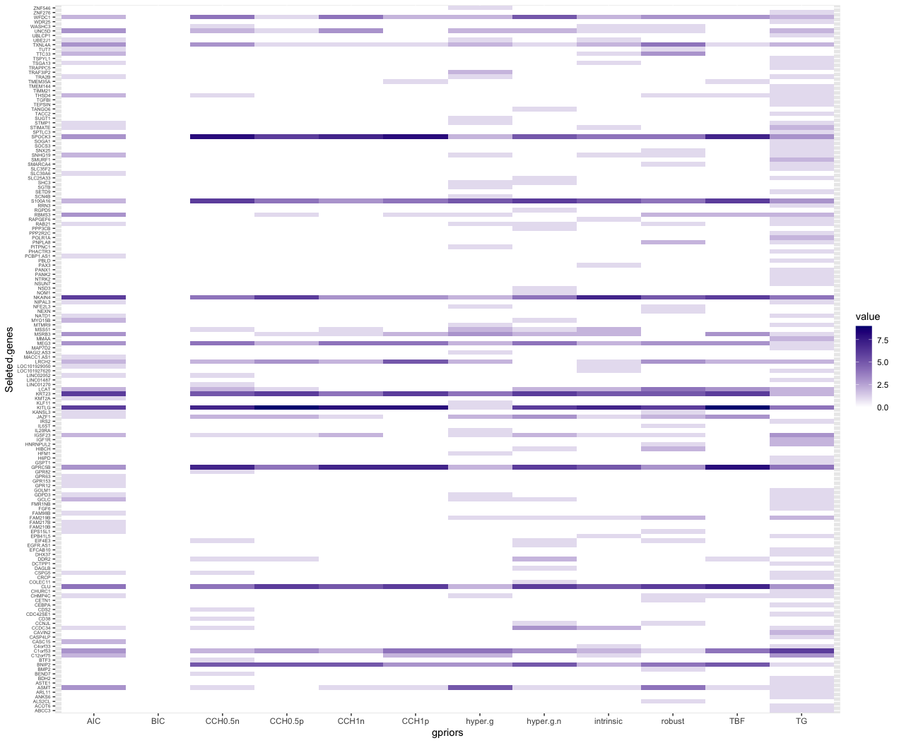
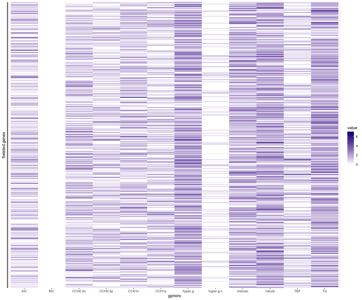
Figure 1 and Figure 2 provide better views of how each g-priors selected genes. Here we can see that a small number of genes are repeated selected by different g-priors model in the beta binomial prior model setting. The gene selection of TG g-prior and AIC are not as condense as other g-priors. In the uniform model prior, it is hard to pick the genes that have high posterior probability.
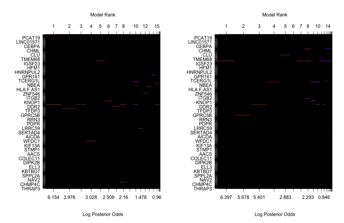
Moreover, we visualized model space of two single model selections og TNB g-prior and hyper p/n g-prior. The color of each line is proportional to the log of the posterior probabilities (the lower x-axis) of that model. However, we found out that in the top of model ranks, only 1 or 2 genes plus the intercept were contained. This means that our best model selected only contains 1 or 2 genes. Therefore, if we want to select more than one genes, we will have to make a criterion on the posterior probability of the coefficients. Here we select 0.01 to control the number of genes in the selection.
Compare with Non-Bayesian Model Selection Methods
Since we want to see the advantages of the mixtures of g-priors, we compared the mixtures g with two regularization models, elastic net and lasso. These are the two well-known methods for the variable selections. Here we used our best performance mixture g models to compare with lasso and elastic net. For lasso and elastic net, we selected $\lambda$ and $\alpha$ (for enet only) by 10-fold cv method. The whole computed process was the same as mixture g model.
In Table 2, we can see that all the models show a relatively good prediction performance. However, the range of gene selection by regularization models is larger than the mixtures g models. This probably accounts to the uncertainty of variable selection methods.
| CCH0.5n | hyper.g.n | TBF | intrinsic | lasso | enet | |
|---|---|---|---|---|---|---|
| Total number of beta | 33.00 | 39.00 | 23.00 | 36.00 | 54.00 | 54.00 |
| cv.error | 0.22 | 0.20 | 0.23 | 0.21 | 0.22 | 0.22 |
| cv.brier | 0.33 | 0.27 | 0.36 | 0.31 | 0.36 | 0.36 |
Discussion
To summarize our findings, for the high dimensional problem, mixtures of g-priors have a relatively good performance in both variable selections and prediction precision if we selected the "right" g-priors and model priors. However, several problems were encountered when we doing the analysis. In the discussion part of the Li and Clyde’s paper, it mentioned that in the non-full rank designs, it is better to choose the sparsity prior or truncated possion distribution prior [4]. However, for the truncated possion prior, the selection of the parameters ($\lambda$ and truncation determination parameter) are crucial to the convergence of the model. Since we did not find out a good method to tune the parameters of truncated prossoin prior, this model prior was not included in this analysis. Moreover, the computational problem in the high dimensional data setting is still existed. In the original data dimension (5357), the running time for this dimension is much longer than only used the 537 top filtered genes. Although we can select the number of unique model sampling, the running time is still considerable. Furthermore, the posterior probability $P(\beta \neq 0 \mid Y)$ is close to 0 for each variable in our original data dimension, which increased the difficulties of variable selection.
Reference
[1] Jennifer A. Hoeting, David Madigan, Adrian E. Raftery, Chris T. Volinsky (1999) "Bayesian model averaging: a tutorial (with comments by M. Clyde, David Draper and E. I. George, and a rejoinder by the authors," Statistical Science, 14(4), 382-417,
[2] Feng Liang, Rui Paulo, German Molina, Merlise A Clyde & "Jim O Berger (2008) Mixtures of g Priors for Bayesian Variable Selection", Journal of the American Statistical Association, 103:481, 410-423, DOI: 10.1198/016214507000001337{.uri}
[3] Hemant Ishwaran, J. Sunil Rao (2005) "Spike and slab variable selection: Frequentist and Bayesian strategies," The Annals of Statistics, 33(2), 730-773,
[4] Yingbo Li & Merlise A. Clyde (2018) Mixtures of g-Priors in Generalized Linear Models, Journal of the American Statistical Association, 113:524, 1828-1845, DOI: 10.1080/01621459.2018.1469992{.uri}
[5] Clyde, Merlise (2020) BAS: Bayesian Variable Selection and Model Averaging using Bayesian Adaptive Sampling, R package version 1.5.5
[6] Zellner A. (1998) On assessing prior distributions and Bayesian regression analysis with gprior distributions. In Bayesian Inference and Decision Techniques: Essays in Honor of Bruno de Finetti, (eds: PK Goel and A. Zellner), 233–243
[7] McCullagh, P., Nelder, J. (1989).Generalized Linear Models, Second Edition. Chapman & Hall. ISBN: 9780412317606
[8] Chen, Ming-Hui, and Joseph G. Ibrahim. (2003) "CONJUGATE PRIORS FOR GENERALIZED LINEAR MODELS". Statistica Sinica, vol. 13, no. 2, pp. 461–476. JSTOR, www.jstor.org/stable/24307144.
[9] Leonhard Held, Daniel Sabanés Bové, Isaac Gravestock (2015) "Approximate Bayesian Model Selection with the Deviance Statistic," Statistical Science, 30(2), 242-257
[10] Gordy, M. B. (1998a), “Computationally Convenient Distributional Assumptions for CommonValue Auctions,”Computational Economics, 12, 61–78.
[11] Abramowitz, M., and Stegun, I. (1970), Handbook of Mathematical Functions - With Formulas, Graphs, and Mathematical Tables, New York: Dover Publications.
[12] Bayarri, M. J., Berger, J. O., Forte, A., and García-Donato, G. (2012), “Criteria for Bayesian Model Choice With Application to Variable Selection,” The Annals of Statistics, 40, 1550–1577.
[13] Wang, X., and George, E. I. (2007), “Adaptive Bayesian Criteria in Variable Selection forGeneralized LinearModels,” Statistics Sinica, 17, 667–690.
[14] Hu, J., and Johnson, V. E. (2009), “Bayesian Model Selection Using Test Statistics,” Journal of the Royal Statistical Society, Series B, 71, 143–158.
[15] Ley, E., and Steel, M. F. (2009), “On the Effect of Prior Assumptions in Bayesian Model Averaging With Applications to Growth Regression,” Journal of Applied Econometrics, 24, 651–674.